246A: Complex Analysis, Notes 1 – Analytic functions, Cauchy’s formula and singularities.

The following series of posts comprises our introduction to complex analysis as taught by Professor Rowan Killip at the University of California, Los Angeles, during the Fall quarter of 2009. Where necessary, course notes have been supplemented with details written by the authors of this website using assistance from Complex Analysis by Elias Stein and Rami Shakarchi. The basic properties of complex numbers will be assumed allowing us to begin with the definition of a holomorphic (or complex-differentiable) function, the central notion in our study of complex analysis.

The basic properties of complex numbers will be assumed, allowing us to begin with the definition of a holomorphic (or complex-differentiable) function, the central notion in our study of complex analysis.

Definition 1.1 Suppose is an open set and . We say is holomorphic (or complex-differentiable) at if there exists We say is holomorphic on if it has this property for all .

We can rewrite this formula in terms of the real and imaginary parts of to surmise the relationship between complex differentiability and real analytic differentiability. Let with and , and write where . Then,

We first notice that this is stronger than the differentiability of the real map in . In the real, multivariable case, the derivative of this map is a linear operator, namely, the Jacobian, ; in our equation above, the matrix on the right hand side is . Clearly, it is endowed with a distinct structure summarized in the following proposition.

Proposition 1.2: The Cauchy-Riemann equations The function is holomorphic at , , with derivative if and only if the functions , where , are differentiable at and

both hold.

Remark There exists a well-known isomorphism between and given by in which it is clear that multiplication by a complex number corresponds to a dilation and rotation via the matrix . Then the above formula indicates that, infinitesimally, a holomorphic map acts like a dilation and a rotation. In particular, if is a holomorphic map such that , then preserves the angle of curves passing through . Such a map is called a conformal (angle-preserving) map. We will discuss conformal maps in further detail later in these notes.

Definition 1.3 A parametric curve is called rectifiable if

Theorem 1.4 If such that is continuous, is open and is rectifiable, then

1. denoted by exists.
2. If then .
3. Given a continuous bijection we have , noting that reversing the direction of the curve changes the sign on the right hand side of the formula above.

Proof: These are immediate consequences of the theory of Riemann integration in one variable and will not be reproduced here.

Theorem 1.5 Goursat’s theorem Suppose is a holomorphic function from the open set to the complex numbers and is a solid, closed triangle inside . Then .

Proof: We begin by giving Cauchy’s proof of Goursat’s theorem, an immediate result of Green’s theorem when is necessarily continuously differentiable. Suppose , then by Green’s theorem, we have that

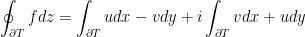
An application of the Cauchy Riemann equations demonstrates that both integrals in the sum are equal to zero, hence as desired.

The classical argument by Goursat uses a stopping-time technique that is both elegant and powerful, albeit not as simple as Cauchy’s proof. On the other hand, it does not require that and is a more general result. (We will eventually learn, however, that a holomorphic function is, in fact, analytic.) To start, we note that it suffices to show that . Next, we subdivide our original triangle into four smaller triangles by bisecting each leg of the triangle and connecting the midpoints with straight lines. This yields four triangles similar to each other and our original triangle . Denote these triangles and in any order. The line integrals over these triangles cancel out over their shared legs, hence . We can then divide each new triangle into four smaller triangles by the process above and claim that To prove our claim, suppose on the contrary, that it does not hold. Then, ; moreover, . Since the are closed and bounded in , they are compact, hence . By hypothesis, is holomorphic at , so that . Then, for some ,

where we denote the perimeter of , (i.e. by and where the integral on the right hand side vanishes as both terms have primitives, or complex-antiderivatives, in . In particular, we have for sufficiently large. This yields the desired contradiction and proves our claim.
Finally, let be the collection of equivalent triangles formed after subdividing our original triangle times. Clearly, they obey the inequality for all . It follows that

as desired.

Remark It is essential that the triangle be contained in . Consider the function integrated along the perimeter of a triangle containing the origin. Then is holomorphic in , and . This theorem can be extended with ease to a path of any other polygon or rectifiable closed curve with one caveat: we must be able to differentiate between the inside and outside of such a curve. More precisely, the curve must be two sided. We are then free to approximate such a curve by a polygon which we can subsequently approximate with triangles.

Goursat’s theorem leads us to one of the most powerful results in complex analysis, the Cauchy integral formula. This result allows us to equate holomorphic functions on sets with integrals over the boundary of these sets. With this isomorphism, one can conclude certain regularity results, in particular, the notion that holomorphic functions are analytic. We begin by considering holomorphic functions defined on sets bounded by the simplest of closed curves: circles.

Theorem 1.5 The Cauchy integral formula Fix and suppose is holomorphic in the set , then,

where .

Proof: Choose and consider the line integral of over the smaller circle . Since this function is continuous in open neighborhoods of this new circle and our original circle (that is, the annulus centered at , containing both circles), we can approximate the integral of this function over both circles arbitrarily closely by integrals over regular -gons, with sufficiently large. Since is open, there exists a simple closed path that connects these -gons. By Goursat’s theorem, the integral of over the closed paths connecting these -gons must be zero. In particular, applying Goursat’s theorem and letting implies

Next, consider and let be a path over the smaller circle. Integrating over this path, we have

This last statement is simply the average of over our smaller circle. Since is continuous throughout , it follows that as . Since was arbitrary, this concludes the proof of our theorem.

Further insight may be gleaned from another proof of the Cauchy integral formula. One attempts to exploit the regularity of the holomorphic function by writing it as an integral of its own difference quotient. In particular, one considers the integral

As above, the integrand is holomorphic away from , (that is, in an annulus centered at ). As above, one equates this integral with one about a small circle around the point . Letting the radius of this small circle tend to zero implies that the above integral is equal to zero. Finally, one computers the Cauchy integral formula directly. This method of proof alludes to a recurrent theme in complex analysis; namely the use of regularity and integral forms to conclude various results.

It may be helpful to note that we’ve used Goursat’s theorem to scale and translate contours in the complex plane without affecting the value of an integral along such a contour. We can derive more general results of this type. In fact, we will see that the statement above, with a similar proof, holds for general Jordan curves.

We now arrive at another fundamental result in the theory of complex variables: that holomorphic functions are analytic. This is a consequence of the Cauchy integral theorem.

Corollary 1.6 Holomorphic functions are analytic. That is, if is holomorphic on , we can express as a power series at each point . Moreover, given and , the radius of convergence of this power series at is at least .

Proof: Fix and . By the Cauchy integral theorem, we have . Let us rewrite the the integrand as follows:

where ; this implies that, for each , and when , the sum above converges uniformly. Hence we can move it outside of the integral and arrive at

as desired. Finally, an application of Hadamard’s formula demonstrates that the radius of the disc of convergence is at least .

Remark Differentiation of the series immediately implies that

from which one can infer the Cauchy estimates:

Corollary 1.7 Morera’s theorem If is continuous on an open set and for each where is a solid triangle in . Then is analytic in .

Proof: Continuity and the fact that allow us to reconstruct the proof of Goursat’s theorem and arrive at its conclusion without requiring, a priori, that be holomorphic. In particular, the Cauchy integral theorem and analyticity follow immediately from the theorems above .

Corollary 1.8 Suppose is a sequence of holomorphic functions that converges uniformly to on compact subsets of . Then, is holomorphic as well. In addition as well.

Proof: Suppose is compact with a solid triangle contained in E. Then, since the are holomorphic, we have

Since uniformly, is continuous and we have

which immediately implies . Since this holds for all compact subsets of , by the preceding theorem it follows that is then analytic on . To prove the final assertion we apply the Cauchy estimates. Suppose again that is a compact subset of . Then, there exists an such that for each , there exists a closed disc . It follows that is a compact subset of as well. By the Cauchy estimates we have

This assertion holds for all , so our conclusion follows as

This result is in stark contrast to situation in the case of real variables. In general, if uniformly with continuously differentiable, it is in general not true that need be differentiable. That the Cauchy integral theorem allows one to represent holomorphic functions as integrals, confers upon holomorphic functions a powerful regularity that leads to many other results. More generally, the use of integral forms plays an important role in analysis because of their regularity. Consider for example the use of the Picard existence theorem for ordinary differential equations. If , then we can conclude the existence of a solution to this differential equation by applying Picard’s iteration and existence to . We can apply the results above to yield further important results.

Corollary 1.9 Liouville’s theorem Suppose is an entire holomorphic function, that is, a function holomorphic on all of , and

for some and . Then is a polynomial with degree not exceeding .

Proof: Since is entire, it can be written as a power series about the origin that converges everywhere on , and it suffices to show that . Let , by the Cauchy estimates we have

For large enough , the bound above implies

The assertion follows as .

The analytic nature of holomorphic functions leads to one of the most profound results in the basic theory of complex analysis: the notion of analytic continuity. This theorem states that if two functions, holomorphic on an open and connected set , agree on an open subset, or even on a convergent sequence of points inside , the two functions must be identical. This tells us that holomorphic functions are in some way fixed by their behavior on an arbitrarily small convergent sequence of points.

Theorem 1.10 Analytic continuity Suppose is a holomorphic function with open and connected and is a sequence of points with a limit point such that vanishes on . Then .

Proof: We prove the theorem by contradiction. If , there exists in a disc of radius about . Then

by continuity and by taking along the sequence . Hence in a small disc of radius about .

Next let . This set must be relatively closed in , since, if it were not, we could find such that . But this is absurd since vanishes in a neighborhood of by the above proof, hence , and is relatively closed. Now, is both open and (relatively) closed, therefore, since it is also connected and non-empty, by a standard result from point set topology, we find that , and that on all of , as we wished to prove.

Remark must be in . If not, we have as a counterexample to the previous theorem. In particular, is holomorphic on vanishes at with but is not identically zero.

A common application of this theorem is as follows. Suppose are holomorphic and agree on a set with an accumulation point. Then on at least one connected component. Note, however, that we must ensure that the hypotheses of this theorem are met; not only do we find a contradiction when but also when our set in question is not connected in the desired sense. For example, suppose that on the principal branch and denotes the complex logarithm of with some other branch cut that starts along the negative real axis near the origin, rises into the second quadrant, curves back down through the third quadrant and deletes the negative imaginary axis below for some . Define in addition as the unique continuous function such that when and via the implicit function theorem. Then is holomorphic. Now, and agree on the right half plane but do not agree everywhere; our difficulty in applying the previous theorem lies in the fact that the region on which they are both holomorphic is disconnected.

The previous theorem allows us, in a very general manner, to infer a great deal about a holomorphic function on an open set by studying its zeros. Such insight leads us to consider the zeros and singularities of functions holomorphic on some , where is a discrete set of singularities in . In fact, investigation of the singularities and zeros of holomorphic functions yields considerable insight into their nature; in particular one concludes the residue theorem, the open mapping principle, and the maximum principle, among others. Our study of the singularities of meromorphic functions motivates the construction and use of the extended complex plane and its geometric interpretation as the Riemann sphere. We proceed by further defining precisely zeros and singularities of meromorphic functions and provide a classification of singularities. Then we continue by providing an interpretation of the extended complex plane and conclude with the Laurent expansion of a meromorphic function.

Definition 1.11 For any function , a singularity of is defined as a complex number such that is defined in a deleted neighborhood of , for an appropriate . For example, suppose on the punctured complex plane (that is, the complex plane deleted at the origin). The origin is then a singularity of the function . By setting , we can extend to the origin. Our resulting function is entire as well as continuous; we call such singularities removable singularities. Alternatively, we can consider the function . This function cannot be extended holomorphically at the origin since as and we say that has a pole at in this case. Lastly, the function on the punctured plane exhibits behavior unlike either of the previous examples. As goes to along the positive real line, approaches infinity. On the other hand, when goes to along the imaginary axis, is bounded, however oscillates rapidly; in this final case, the origin is called an essential singularity. These three cases exhaust all possibilities.

Definition 1.12 A complex number is a zero of the function if . Analytic continuity demonstrates that if is the set of zeros for a function holomorphic on the elements of must be isolated. In this case, we call a discrete set.

Theorem 1.13 Suppose is holomorphic in the open, connected set and has as a zero and does not vanish identically in . Then there exists a neighborhood of , a non-vanishing holomorphic function and a unique, non-zero, positive integer such that

for all .

Proof The proof is immediate. Since is not identically zero in , it follows from the power series expansion , of , that there exists an and satisfying the conclusions of the theorem. Alternatively, if we suppose that has a pole at of order , applying this theorem to the function proves that we can write with and as above.

We can infer more about functions exhibiting singularities; first we note that we can decompose such functions into a holomorphic and principal part. In fact, these functions are holomorphic inside an annulus about their singularities. An application of Cauchy’s integral formula proves that there exists a generalization of this decomposition, the Laurent expansion. With this framework, properties of analytic functions, both entire functions and those with singularities can be more easily studied. First, two simple theorems demonstrates that functions with removable singularities admit a fairly straight-forward description as a result of Riemann’s removable singularity theorem. Our prior example of a function with an essential singularity exhibited erratic behavior near it; we find that this is true in general, as the Casorati-Weierstrass theorem demonstrates.

Theorem 1.14 Suppose is an open neighborhood of , without loss of generality, and suppose is holomorphic on obeying

on with and . Then, there exists a holomorphic function and coefficients such that

 

The sum above is called the principal part of . When , this result is called the Riemann removable singularity theorem.

Proof: First consider the case . We find that is bounded on . Consider the function . As a result of our boundedness hypothesis, and exist, and it follows immediately that is holomorphic on . In addition, vanishes to at least second order at zero. An application of the previous theorem implies is holomorphic on all of , from which our assertion follows. Clearly, the singularity at the origin must be removable. Now, if , note that ; an application of our prior result to implies

for some function holomorphic on . Expanding in its power series about and dividing by on both sides concludes the proof of our theorem.

One should note that this result is essentially equivalent to the conclusion of the theorem proceeding it. In particular, if is a meromorphic function with a pole at of order , then, can be decomposed into the sum of its principal part and a holomorphic function. Equivalently, .

Theorem 1.15 Casorati-Weierstrass Suppose is holomorphic in with an essential singularity at . Then is dense in .

Proof: Rather, suppose is not dense in . Then there exists and such that . Therefore, if we let

we find that on . By the Riemann removable singularity theorem, must be holomorphic on ; that is, must be holomorphic at or exhibit a pole at , both of which contradict the nature of the singularity at . Hence, must be dense in .

Theorem 1.14 allows one to decompose a function exhibiting a pole singularity into an analytic and principal part. This is true in general, as the Laurent expansion allows one to expand any complex function into a convergent analytic and principal part, the latter with a possibly infinite number of terms. First, we require a lemma. It suffices during the following discussion to consider without loss of generality, functions analytic on an annulus about the origin.

Lemma 1.16 Let with be an annulus and suppose is analytic. Furthermore, suppose such that . Then,

Proof: The lemma is an immediate result of the Cauchy integral formula and was used in its derivation.

Proposition 1.17 Laurent expansion Any complex function that is analytic on an annulus admits as a decomposition

with and analytic, where and are open discs of radius and , centered at the origin. If vanishes at the origin, then the expansion is unique. In the latter case, is called the principal part of the Laurent expansion of .

Proof: We first address the notion of uniqueness. If has two different Laurent expansions, their difference is the Laurent expansion for the zero function, hence it suffices to prove uniqueness for the expansion of the zero function. Suppose . This function is analytic on all of and is clearly bounded, hence, by Liouville’s theorem, is constant. This implies that and are both identically zero, thus guaranteeing that the Laurent expansion of the zero function is unique.

As we discussed earlier, the exploitation of integral forms plays a significant role in analysis. Our construction mimics the derivation of the power series expansion for analytic functions. In particular, we exploit the regularity conferred to by its analyticity and write as the primitive of a function much like its own derivative, in other words, an integral form. Provided the necessary assumptions are met, one can then study by manipulating its integral form.

Fix such that and let be defined by

This function is analytic on and has a removable singularity at by the Riemann removable singularity theorem. From this and our prior lemma we find that

In other words, we have

Because lies outside the small circle the function is on open neighborhoods containing this circle. Therefore, we have

On the other hand, the function is not analytic on open neighborhoods containing the large circle hence,

from which it follows that

This is our desired Laurent expansion. We find that

where and,

where . These functions are both analytic, hence we can write them as power series. Therefore,

and

Finally, if we denote , we conclude

In order to continue with a thorough treatment of complex functions and their singularities, we introduce the extended complex plane, denoted henceforth by and defined by appending the point at infinity to . More precisely, for large values of , we consider the function and identify the behavior of at infinity by the corresponding behavior of at the origin. For example, if is holomorphic for large , then is holomorphic in a deleted neighborhood of the origin. Similarly, the function has a pole at infinity if has a pole at the origin; other behavior of at infinity is defined synonymously.

The extended complex plane admits a powerful geometric description which we consider next.

Definition 1.18 The extended complex plane the Riemann sphere and stereographic projections

Let and identify the -plane with . Furthermore, let be the unit -sphere centered at the origin. Denote by its top most point , that is, . Then, for any point , we can draw a straight line connecting and intersecting the -plane at a point , which we write, in the notation of complex analysis as . Alternatively, given any point on the -plane, say, , there exists a unique point along the vector . Intuitively, we can see that such a correspondence must be bijective. In particular, it is clear that there is a bijective correspondence between and . Now suppose , that is, let the point go to infinity on the -plane. The point then moves arbitrarily close to , and we find that there exists a correspondence between the point at infinity in and the north pole of the unit sphere, . Hence we can identify with the -sphere, otherwise known as the Riemann sphere. The addition of the point at infinity to is called the one-point compactification of since it takes to the compact set by adding one point. In particular, the stereographic projection is given by the map

with inverse

A few fairly simple algebraic (or geometric) manipulations demonstrates that these maps are conformal, assuring us of the validity of our prior discussion. With this construction in mind, we turn to the study of meromorphic functions in our subsequent notes.