Ross Recovery

In this post, we discuss the interesting paper by the late Steve Ross,”The Recovery Theorem”, in which a method is proposed to disentangle the risk aversion component from the subjective probability measure from state prices. In particular, a method is proposed to back out the market’s forecast of returns (a distribution over returns) from option prices.

Overview

State prices are the product of risk aversion—the pricing kernel—and the natural probability distribution. From derivatives prices we can observe distribution of state prices. The question then becomes: can we separate the markets probability distribution over returns and risk aversion?  For example, we would like to know, given forward rates, how much of the rate is due to the market’s forecast and how much is a risk premium. In models with a representative agent, this is equivalent to knowing both the agent’s risk aversion and the agent’s subjective probability distribution, neither of which is observable but instead, inferred from calibrating market models.

Ross finds a decomposition of state prices into a risk adjustment and the natural probability distribution assuming that the pricing kernel is irreducible and transition independent (defined below). He calls this a recovery theorem. He proves his recovery theorem in two settings: finite state space, and a multinomial (potentially countably infinite) state space. The decomposition then allows us to express the market transition probabilities in terms of the stochastic discount factor and state prices, both of which can be estimated. The proof of the finite state space is essentially a fairly straight forward application of the Perron-Frobenius theorem. The proof of the result in the multinomial setting requires an additional assumption and follows from an unclear proof by (implicit) induction.

As a corollary to the recovery theorem, the subjective discount rate is shown to be bounded above by the largest interest factor. In addition, in the finite state case, if the riskless rate is state independent, then pricing is shown to be risk neutral. This is a very surprising result and in fact does not hold true for the countably infinite multinomial case. At the moment, I do not have good intuition for this result, but Ross claims that it is an artifact of having a finite irreducible process for a state transition (see bottom of pg 623).

Ross then goes on to demonstrate the recovery theory in two different ways. First, he shows for a “static” example, that given both the utility function (CRRA in his example) and the stock price distribution (lognormal) that using the recovery theorem, one can recover the natural probability measure using the pricing kernel (SDF) and the state prices. In the given example, the utility function and the price distribution are used to derive the expressions for the SDF and the state prices (through the Black-Scholes-Merton formula). He then calibrates the standard deviation and mean return of the price process (price distribution) to market data and shows that the resulting recovered transition probability distribution coincides with the lognormal distribution. This section (Section IV) proves to be deeper than just a verification of the theorem for an example.  First, Ross points out that although the theorem was proven for the discrete and multinomial cases, it still seems to recover with a continuous distribution when considering a static problem (moving from one known initial state to an unknown state). However, once the dynamic problem is considered where one first transitions from a known state to an unknown state, then from the unknown state to another unknown state (from time 0 information set perspective), problems arise in that no implicit truncation of the distribution can be used. Details on this will be given below.

In section V, the recovery theorem is applied to the S&P 500 index to recover the market transition probabilities on April 27, 2011. What is remarkable about the recovery method is that it doesn’t need a training set. That is no historical data is explicitly needed to recover the distribution. The only place that Ross makes use of historical data is for the sake of comparison. Using historical returns, he constructs a bootstrapped histogram of returns and compares it to the recovered histogram of returns.

In the last section, a “model-free” test of the efficient market hypothesis (EMH) is proposed that essentially bounds the R^2 one can get from a factor model that would still be consistent with the EMH. Thus, any test of an investment strategy that uses publically available information and has the ability to predict future returns with R^2 > 10% would be a violation of efficient markets independent of the specific asset pricing model being used, subject to the maintained assumptions of the recovery theorem. Of course, such a strategy must also overcome transactions costs to really be a violation. His bound doesn’t take into account any transactions costs.

Basic Framework (§ II-III)

The basic framework is a discrete-time world with asset payoffs at time $ latex T$, contingent on the state θ∈Ω. From the fundamental theorem of asset pricing (FTAC), no arbitrage implies the existence of a positive state space prices, p(θ) (or in more general spaces, a price distribution function ). The current value of an asset paying in period T is given by

Where an asterisk denotes the expectation with respect to the martingale measure and where the pricing kernel, is the Radon-Nikodym derivative of with respect to the natural (subjective) measure, or in the case of continuous distributions, , where is the subjective pdf. The risk neutral probabilities are given by

Our first assumption is that the asset value follows a Markov process. Ignoring the effects of the time value of money temporarily, the (martingale) transition density function, , must satisfy the Chapman-Kolmogorov equation:

for any The idea behind (3) is that the probability of transitioning from state to from time 0 to time T can be decomposed into the total probability of first transitioning to some arbitrary state at the intermediate time t and then transitioning to the state time T. Furthermore, since Q is a martingale measure, we also get time homogeneity which is why we can view everything from the time zero perspective, i.e. instead of thinking about the transition density from t to T we can just think about the transition density from 0 to T-t.

Taking back into account the time value of money, and making the second assumption that the process is time homogenous, the state price distribution is given by

Under the Markov assumption and assuming a continuous distribution for illustrative purposes, the kernel (state price per unit of probability (density)) as

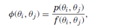
In the familiar world of a representative agent with additive time-separable preferences we get

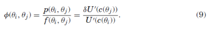
Most likely inspired by this form, Ross imposes the third assumption of transition independence on the kernel:

More general preferences than additive time-separable utility satisfy this form such as Epstein-Zin recursive preferences. At this point, we should pause to reflect how much this assumption has bought us. If we look at the LHS, in discrete time and state space world with m states, it will be a matrix with up to degrees of freedom whereas the RHS just has degrees of freedom (h takes on m different values, and is also unknown). Thus, we reduced our search from to .

From (9) and (10) above, we obtain an expression for state prices

In what follows, we specialize our discussion to a discrete state space model. Let

where or more generally, is any positive function of the state. Rewriting (11) in matrix form, we get

We can then express the natural transition matrix F as

In addition, since F is a transition matrix, its rows must sum to one, we have the additional set of m constraints:

Rearranging, we get the characteristic root problem:

Finally we make our fourth assumption that P is irreducible which allows us to use the Perron-Frobenius Theorem. One of the results of the theorem is that all non-negative irreducible matrices have a unique positive characteristic vector, z and associated eigenvalue which corresponds to our lambda. This essentially gives us the main theorem:

From this, we have that is the maximum characteristic root of the price transition matrix, . Furthermore, another result of Perron-Frobenius gives us that this root is bounded above by the maximum row sum of , which are the interest rate factors.

Furthermore, if the riskless rate is the same in all states, we get the surprising result

Multinomial Recovery (§ III)

Here Ross extends the theorem to an infinite horizon multinomial Lucus tree setting. It’s useful to note that three of the four sufficient conditions discussed hold in this setting. First, it is still a Markov process. Second, transition independence is directly assumed from assuming time additive utility set-up so that state prices will have the form of (10). Third, irreducibility still holds as any state almost surely is revisited in finite time. The assumption which is not met is the time independence assumption. The payoffs of the tree grow (or shrink) with time so it is another state variable. Under these assumptions we get Theorem 4:

An Example, Comments, and Extensions (§ IV)

In this section, Ross goes on to demonstrate the recovery theory in two different ways: first, he shows for a “static” example, that given both the utility function (CRRA in his example) and the stock price distribution (lognormal) that using the recovery theorem, one can recover the natural probability measure using the pricing kernel (SDF) and the state prices. In the given example, the utility function and the price distribution are used to derive the expressions for the SDF and the state prices (through the Black-Scholes-Merton formula). He then calibrates the standard deviation and mean return of the price process (price distribution) to market data and shows that the resulting recovered transition probability distribution coincides with the lognormal distribution. This section (Section IV) proves to be deeper than just a verification of the theorem for an example.  First, Ross points out that although the theorem was proven for the discrete and multinomial cases, it still seems to recover with a continuous distribution when considering a static problem (moving from one known initial state to an unknown state). However, once the dynamic problem is considered where one first transitions from a known state to an unknown state, then from the unknown state to another unknown state (from time 0 information set perspective), problems arise in that no implicit truncation of the distribution can be used (see pg 632-633).

Applying the Recovery Theorem (§ V)

In this section, Ross relying on a rich market for European options to numerically approximate the state prices. To do so, we first note that a European call price with strike K and time of maturity T can be expressed as

From Breeden and Litzenberger (1978), and intuitively from naively applying the FTC, we have which is approximated numerically from the second differences of the observed call prices.

To apply the Recovery Theorem, we first have to estimate the state price transition matrix.

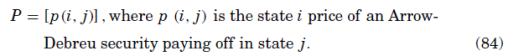
Now, to index the states, we think of there being m possible states at any time 0 and time T – there is no growth in this formulation as in the multinomial model. Ross’s notation in this section is pretty terrible, but for the sake of comparability with the paper I will maintain it and do my best to explain it. First, we denote each row of the transition matrix from time 0 to T, , by where c denotes the current state at time 0.

The arguments denote the state at time —the current state notation is suppressed in the vector list. This same notation is used in (83). Next, we denote P as the one period transition matrix. . One of the rows of P we get by using (83) to find the entries of (cf. (85)). To find the rest of the entries of P, we use the following Markovian relationship

where m is the number of states. This is a system of equations in the variables , and since we know current state prices, we can solve this.

Figure 2 show the recovered densities vs the bootstrapped ones. Ross points out that the recovered density has a fatter left tail and suggests that this provides support to the recovery method as we should expect the subjective density to have a fatter left tail (fear of disaster) than the actual probability density.

Testing the Efficient Market Hypothesis (§ VI)

In Ross (2005), an alternative test to testing the EMH by finding an upper bound to the volatility of the pricing kernel is proposed. The recovery method allows us to find a number for this upper bound. In particular, from the Hansen-Jagannathan bound there is a lower bound on the volatility of the pricing kernel, :

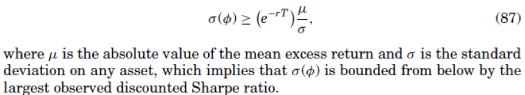
Recovery gives us an estimate . Next, we can decompose excess returns, , on an asset or portfolio strategy as (see Ross(2005))

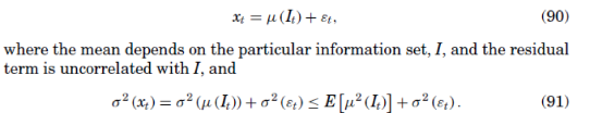
Rearranging and recalling (87) yields an upper bound on the of the regression:

Given the estimate of and interest rates at 0, this means that 10% of the annual variability of an asset (or portfolio) return is the maximum amount that can be attributed to movements in the pricing kernel with 90% idiosyncratic in an efficient market.

Bubbles and Crashes: The Local Martingale Characterization of Asset Price Bubbles

We resume our Bubbles and Crashes series with this post discussing the recent influential works of Robert Jarrow and Phillip Protter on the characterization of bubbles as Local Martingales: The Local Martingale Characterization of Bubbles pdf

246A: Complex Analysis, Notes 2 – Meromorphic Functions and Properties of Analytic Functions

We continue with a discussion about meromorphic functions and the properties of analytic functions. Later notes will consider the Riemann mapping theorem, harmonic functions and the Dirichlet problem among other topics.

Definition 2.1 A function on an open set is meromorphic if there exists a discrete set of points such that is holomorphic on and has poles at each . Furthermore, is meromorphic in the extended complex plane if is either meromorphic or holomorphic at . In this case we say that has a pole or is holomorphic at infinity.

By collecting results from the previous section, we are immediately led to the following proposition regarding the Laurent expansions of complex valued functions.

Proposition 2.2 Let be the discrete set of singularities of a complex function where is an open set in . For a fixed , suppose the Laurent expansion for in an annulus about is given by . Then,

1. The function has a removable singularity at if and only if for all .
2. The function has a pole at if and only if there exists with such that for all ; that is, the Laurent expansion of about has only finitely many negative terms.
3. The function has an essential singularity at if and only if the Laurent expansion of about has infinitely many negative terms.
4. Furthermore, is meromorphic on the extended complex plane if and only if there exists such that for .

246A: Complex Analysis, Notes 1 – Analytic functions, Cauchy’s formula and singularities.

The following series of posts comprises our introduction to complex analysis as taught by Professor Rowan Killip at the University of California, Los Angeles, during the Fall quarter of 2009. Where necessary, course notes have been supplemented with details written by the authors of this website using assistance from Complex Analysis by Elias Stein and Rami Shakarchi. The basic properties of complex numbers will be assumed allowing us to begin with the definition of a holomorphic (or complex-differentiable) function, the central notion in our study of complex analysis.

The basic properties of complex numbers will be assumed, allowing us to begin with the definition of a holomorphic (or complex-differentiable) function, the central notion in our study of complex analysis.

Definition 1.1 Suppose is an open set and . We say is holomorphic (or complex-differentiable) at if there exists We say is holomorphic on if it has this property for all .

We can rewrite this formula in terms of the real and imaginary parts of to surmise the relationship between complex differentiability and real analytic differentiability. Let with and , and write where . Then,

We first notice that this is stronger than the differentiability of the real map in . In the real, multivariable case, the derivative of this map is a linear operator, namely, the Jacobian, ; in our equation above, the matrix on the right hand side is . Clearly, it is endowed with a distinct structure summarized in the following proposition.