Bubbles and Crashes: A Survey of the Efficient Market Hypothesis, Part II

1. Empirical Tests of the Efficient Market Hypothesis and their Results

The models developed so far provide the theoretic basis for our study. We have clearly defined efficient markets and discussed a paradox in their construction, the joint hypothesis problem. We have used the language of probability theory to imbed rigor into our definition. But, we also find that much of the inspiration for these definitions arose from experience. Germinated by a broad intuition for the structure of asset returns and supported by practical experience with traders and trading, the theory is something of a hybrid: equal parts practice and principle. It was sculpted by finely-tuned economic insight, and followed statistical study or grew alongside it. Mathematical rigor was one fiber in the thread of its development.

Historically, the empirical study of the efficient market hypothesis focused on whether prices fully reflect particular subsets of information, while the unpredictability of stock market returns played a lesser role. Weaker forms of the EMH were tested first. The first subset of information considered was that of past prices, and financial economists sought to determine the validity of the weak form efficient market hypothesis. The next subset of information considered concerned the speed at which asset prices adjusted to news and other information as well as past prices; these studies tested the semi-strong form of the hypothesis. Later work considered past prices, fundamental data, news, and insider information, in an attempt to study the strong form efficient market hypothesis.

Today, support for the EMH is not without caveat; its intemperate defense is akin to ideology rather than social science. Substantial empirical and theoretic research has demonstrated its weaknesses. But neither has it been removed nor replaced. Revisions have strengthened it and endowed it with nuance. Modern perspectives reiterate its usefulness as a central tool in the study of financial market, while description of its failings sharpen the edges of its impression. In fact, it holds up rather well to a variety of introductory tests, as we will soon see. (We will defer criticism of these tests until later in order to preserve the chronology of the literature.)

1.1. Random Walks and Weak Form Tests

While a number of tests of the efficient market hypothesis centered on the random walk of asset price returns, many of these results can, in fact, be interpreted as tests of fair game expected return models instead. More general, and as a result, more encompassing, this interpretation supplies a better perspective of the breadth of the EMH.

Around the 1970s, much of the empirical literature focused on the serial covariance of asset returns, in particular, for random walk models. If, in fact, asset price changes obey a random walk, then by definition, their serial covariances must be zero: each asset price change is independent of the others, hence their covariance is zero. Fair game models behave similarly.

If are random variables, their serial covariance is given by

where is a density function. Now, if is a fair game random variable, its unconditional expectation is zero, and

in other words, the serial covariance is zero. It follows immediately that the observations of a fair game variable are linearly independent.

However, the fair game model does not imply that the serial covariances of one-period returns are zero. As before, let denote the deviation from the expected return of the asset at time . That is, let

Then the serial covariance of subsequent one-period returns are given by

But (1) does not imply . In other words, deviation from the conditional expectation at a specific time period may be fair game, but the conditional expectation itself may be dependent on the previous period. In the stock market, this does not seem to pose a problem; empirical results demonstrate that variation introduced by minimizing this fact is trivial compared to other sources of variation. In the market for treasury bills, however, more care is required, as we will later discuss.

Empirical results confirm that the serial correlations between successive changes in the natural logarithm of price for each of the thirty stocks of the Dow Jones Industrial Average from about the end of 1957 to the end of 1962 are always close to zero.

But we soon see problems. Fama says “looking hard, one can probably find evidence of statistically ‘significant’ linear dependence [in these results].” The correlation coefficients obtained from these studies indicate that a linear relationship with laggard price changes may account for about percent of the variation in the current price change. One of course wonders what fraction of variation a non-linear model might prescribe.

Other research analyzes the success of trading rules that would profit from serial correlation in price changes. Sidney Alexander’s paper, Price Movements in Securities Markets exhibits the failure of a number of such trading systems, such as the filter. Although he finds evidence against the random walk hypothesis–the independence assumption appears unlikely–his results largely confirm the fair game efficient market hypothesis.

Other Tests of Independence in the Random Walk Literature The evidence demonstrates that it is preferable to consider the random walk hypothesis as a special case of the fair game model. If one-period returns are independent and identically distributed (i.i.d.), within the fair game model, then the random walk hypothesis will also hold. As a special case, however, its conditions are more stringent and its assumptions more sensitive. We expect that empirical data will violate the random walk hypothesis often, yet both its robustness and its failures will serve to expose the underlying structure of the market. In a sense, it will help delineate the concrete structure within markets from the ethereal and vague.

One departure from the pure independence assumption of the random walk hypothesis concerns the expected magnitude of daily price changes. Large price changes tend to be followed by large price changes with some regularity. The direction of these changes, however, is seemingly random. This contradicts the random walk hypothesis, but not the fair game model. It is believed that, as information enters markets, participants may overreact (or fail to react). Since subsequent changes are random in direction, this reaction has little bearing on the ultimate trajectory of prices. Interestingly enough, this is sufficient for the expected return efficient market model.

Distributional Evidence Previous results have established that whatever dependence seems to exist in series of historical returns, it appears virtually impossible to use this dependence to make reliable, profitable predictions about the future evolution of returns. There is little evidence that would overturn the random walk hypothesis, at least as an approximation.

At the time of the publication of Fama’s review paper, much of the current empirical research concerned the statistical distribution of price changes. Even now, understanding the distribution of returns remains important. The shape that returns take strongly influences the statistical tools available for research, the theoretic tools economists regularly use to study the structure of financial markets, and the interpretation of these results.

Louis Bachelier was the first to propose that price changes adhered to a normal distribution. He assumed that price changes from moment to moment were independent and identically distributed (i.i.d.) random variables with finite variance. If transactions are numerous, and uniformly distributed, then an application of the Central Limit Theorem implies that prices changes will be normally distributed. Subsequent studies were far less certain. Osborne, Moore and Kendall found that, while prices appeared somewhat normally distributed, the tail ends of the distribution function were larger than expected. The distribution of price changes was, in fact, fat-tailed: extreme price changes occurred far more often than the normal distribution would indicate. This particular observation, while known to a number of financial economists in the 1970’s, has gained notoriety in recent years. Fat-tailed distributions (and large deviation theory, of which it is an element), underlie much of the popular and academic discussion of stock market crashes and large-scale political events. No more bold or vociferous a writer has emerged as Nassim Nicholas Taleb. His books, The Black Swan and Fooled By Randomness, discuss these distributions with bravado.

Taleb’s oft cited mathematician, Benoit Mandelbrot, became influential among financial statisticians in the 70’s precisely for his weaker description of price distributions. He proposed that price changes obeyed a more general category of distribution, stable class distributions, of which the normal distributions were a subset. Unfortunately, economists have been reluctant to accept his results due to the wealth of techniques available for studying series of normally distributed random variables; the infrastructure available in probability theory itself permits the application of a variety of limit theorems and laws of large numbers. When contrasted with the “relative paucity” of techniques for non-normally distributed random variables, the reason for this preference become clear. More salient, however, is the concern that the inability of probability theorists to tame non-normal random variables may hint at a similar inability of financial economists to thoroughly tame randomness within markets.

Fair Game Models in the Treasury Bill Market As we saw earlier, fair game properties of the general expected return models apply to the variable

For common stock it is appropriate to assume 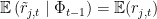, since is so much greater than changes in the expected value of that the latter can be safely ignored. This does not hold, however, for treasury bills. Testing the T-Bill market for efficiency will require more nuance, and an understanding of the economic theory that describes the evolution of treasury returns over time.

Richard Roll uses a variety of models in order to test for efficiency. In these models, describes the rate observed from the term structure at time for one week loans to begin at ; can be thought of as the “futures” rate of these bills. This implies

however, the random variable is observed a period earlier, at the time . Furthermore, is the “Liquidity premium” in . That is,

the one-week “futures” rate at time is equal to the expected “spot” rate at time for plus a “liquidity premium.” In Roll’s theories of term structure, we also have

Empirical tests demonstrate that is generally non-zero, and is slightly more likely to be positive, indicating that investors are paid a premium for bearing interest rate uncertainty. Moreover, under models in which the liquidity premium is non-zero, Roll’s testing indicates that the market for Treasury bills is nearly efficient; the are serially independent.

Tests of a Multiple Security Expected Return Model So far, our discussion has concerned so-called “single security” tests, in which we’ve sought to determine the accuracy of an individual asset’s price; we have considered whether profitable trading systems exist for single securities. Our answers have taken a variety of forms, and we have yet to explore empirical results of the other versions of the EMH. We are led immediately to another question: are portfolios of securities necessarily efficient? Are the returns of groups of securities appropriately priced in relation to each other? These questions motivated Sharpe and Lintner in their research; this work eventually became the foundation for modern portfolio theory.

Consider the expected return of the security from time to time , and suppose are the returns on a hypothetical risk-free asset and on a “market portfolio” respectively, where the later is composed of every asset in our market, weighted in proportion to their total market value. Then,

where is the standard deviation of the return on , and to covariance is as written. As written, it is clear that the model is limited to returns with finite variance, but later research has extended it to series of returns with infinite variance and stable distribution; in addition, it has been extended to multi-period settings as well.

In this model, each investor holds some combination of the risk-free asset and the market portfolio; as a result, “the risk of an individual asset can be measured by its contribution to the standard deviation of the return on the market portfolio.” In other words, the risk of an individual asset is equal to

Indeed, since

it follows immediately that the risk of an individual asset is equal to its “weight” in the sum above.

The work of Fama, Fisher, Jensen and Roll continued with this line of research, developing the so-called “market model” given by

where, much like before, is the rate of return on security at time , is the corresponding rate of return on the market index , are fixed coefficients for each security , and is a random noise term with mean equal to zero.

Econometric analysis demonstrates that the equation above is well-defined as a linear regression model, the parameters remain fairly constant over long periods of time, and and appear to be serially independent. These are the very criteria for the initially stated expected returns efficient market model. Studies find that the data agree with the market model specified in such a way that we can be fairly confident securities are efficiently priced in relation to one another. Furthermore, taking the expectation of both sides, we find

a lucid description regarding the evolution of expected returns.

Simple arithmetic, then, is enough to relate these results with studies of the Sharpe-Lintner model. Rearranging , we find

since , that is, the risk-free rate is an element of the information set at time , we note that

and

A few strong assumptions are necessary to construct the relationship. If the variance and covariance above are constant for all , then ; in fact, in this case, is the least squares estimate of . Finally, if is constant over and can be approximated by some suitable index , with

the market model and the Sharpe-Lintner models are equivalent. Further econometric studies of Sharpe-Lintner would then reiterate that not only do these models describe portfolio evolution well, but that securities are priced appropriately in relation to one another.